Frogs, flies, and Julia

Here's the July PuzzlOR question, courtesy of John Toczek. Now that the competition is over, let's go to town.

Frog fly game image

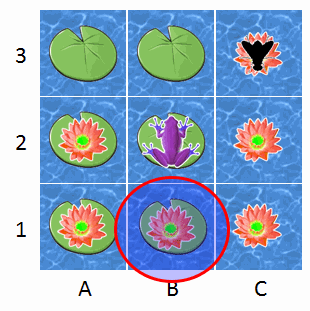
A frog is looking to catch his next meal just as a fly wanders into his pond. The frog jumps randomly from one lily pad to the next in hopes of catching the fly. The fly is unaware of the frog and is moving randomly from one red flower to another.

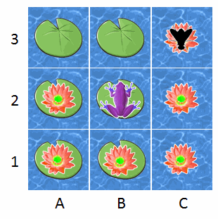
The frog can only move on the lily pads and the fly can only move on the flowers. The interval at which both the frog and the fly move to a new space is one second. They never sit still and always move away from the space they are currently on. Both the frog and the fly have an equal chance of moving to any nearby space including diagonals. For example, if the frog were on space A1, he would have a 1/3 chance each of moving to A2, B2, and B1.

The frog will capture the fly when he lands on the same space as the fly.

Question: Which space is the frog most likely to catch the fly?

This is another Markov chain puzzle, similiar in some ways to the post about modeling chutes and ladders as a Markov chain or the spy catcher puzzle. The twist here is that instead of being a static absorbing Markov chain or a single random process, the game ends when two discrete random processes converge on the same state.

Lately, I've been playing with the Julia language, so I'll do this one using Julia.

Julia logo

Thanks to the awesome IJulia library, we don't have to give up the IPython notebook. For me, that's a huge selling point.

Setting up the problem

Let's number these squares:

Frog fly game numbered

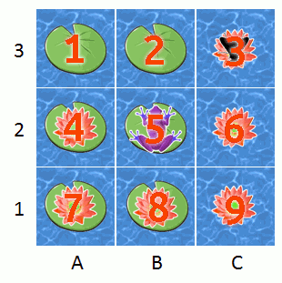
Now that we have consistent way to refer to the states that the fly and the frog can be in, we will create adjacency matrices that define how they are able to move.

By convention, element $M_{ij}$ of an adjacency matrix tells you if state $j$ (the column) is reachable from state $i$ (the row). For example, if the fly is on square 9 then the only two adjacent nodes with flowers that it can reach next are squares 6 and 8. Therefore, in row 9 of the flower adjacency matrix, only the 6th and 8th elements are equal to one (indicating adjacency) while the rest are equal to zero (meaning they are unreachable from the current state).

In [1]:
# the frog's possible transitions
adj_frog =  [0  1  0  1  1  0  0  0  0;
             1  0  0  1  1  0  0  0  0;
             0  0  0  0  0  0  0  0  0;
             1  1  0  0  1  0  1  1  0;
             1  1  0  1  0  0  1  1  0;
             0  0  0  0  0  0  0  0  0;
             0  0  0  1  1  0  0  1  0;
             0  0  0  1  1  0  1  0  0;
             0  0  0  0  0  0  0  0  0]

adj_fly = [0  0  0  0  0  0  0  0  0;
           0  0  0  0  0  0  0  0  0;
           0  0  0  0  0  1  0  0  0;
           0  0  0  0  0  0  1  0  0;
           0  0  0  0  0  0  0  0  0;
           0  0  0  0  0  0  0  1  1;
           0  0  0  1  0  0  0  1  0;
           0  0  0  1  0  1  1  0  1;
           0  0  0  0  0  1  0  1  0]
Out[1]:
9x9 Array{Int64,2}:
 0  0  0  0  0  0  0  0  0
 0  0  0  0  0  0  0  0  0
 0  0  0  0  0  1  0  0  0
 0  0  0  0  0  0  1  0  0
 0  0  0  0  0  0  0  0  0
 0  0  0  0  0  0  0  1  1
 0  0  0  1  0  0  0  1  0
 0  0  0  1  0  1  1  0  1
 0  0  0  0  0  1  0  1  0

We'll also define a function to normalize the rows, and turn them into conditional probabilities. (Much more on this in the spy catcher post.)

In [2]:
function stochastic_matrix_from_adjacency_matrix(M)
    
    # initialize a Float64 matrix of same size as M
    P = zeros(size(M))
    
    # normalize each non-zero row by dividing by sum of row
    for i in 1:size(P, 2)
        if sum(M[i, :]) > 0
            P[i, :] = M[i, :] / sum(M[i, :])
        end
    end
    
    P
end
Out[2]:
stochastic_matrix_from_adjacency_matrix (generic function with 1 method)


Using this function, we'll get the stochastic matrices for the fly and frog.

In [3]:
P_fly = stochastic_matrix_from_adjacency_matrix(adj_fly)
Out[3]:
9x9 Array{Float64,2}:
 0.0  0.0  0.0  0.0   0.0  0.0   0.0   0.0  0.0 
 0.0  0.0  0.0  0.0   0.0  0.0   0.0   0.0  0.0 
 0.0  0.0  0.0  0.0   0.0  1.0   0.0   0.0  0.0 
 0.0  0.0  0.0  0.0   0.0  0.0   1.0   0.0  0.0 
 0.0  0.0  0.0  0.0   0.0  0.0   0.0   0.0  0.0 
 0.0  0.0  0.0  0.0   0.0  0.0   0.0   0.5  0.5 
 0.0  0.0  0.0  0.5   0.0  0.0   0.0   0.5  0.0 
 0.0  0.0  0.0  0.25  0.0  0.25  0.25  0.0  0.25
 0.0  0.0  0.0  0.0   0.0  0.5   0.0   0.5  0.0 
In [4]:
P_frog = stochastic_matrix_from_adjacency_matrix(adj_frog)
Out[4]:
9x9 Array{Float64,2}:
 0.0       0.333333  0.0  0.333333  0.333333  0.0  0.0       0.0       0.0
 0.333333  0.0       0.0  0.333333  0.333333  0.0  0.0       0.0       0.0
 0.0       0.0       0.0  0.0       0.0       0.0  0.0       0.0       0.0
 0.2       0.2       0.0  0.0       0.2       0.0  0.2       0.2       0.0
 0.2       0.2       0.0  0.2       0.0       0.0  0.2       0.2       0.0
 0.0       0.0       0.0  0.0       0.0       0.0  0.0       0.0       0.0
 0.0       0.0       0.0  0.333333  0.333333  0.0  0.0       0.333333  0.0
 0.0       0.0       0.0  0.333333  0.333333  0.0  0.333333  0.0       0.0
 0.0       0.0       0.0  0.0       0.0       0.0  0.0       0.0       0.0


Now let's write some functions to simulate the frog and fly game.

In [5]:
function move(state, P):
    """
    Given a current state and a transition matrix, execute one
    transition.
    
    state -- an int representing the current state
    P -- the stochastic matrix
    """

    # find stochastic vector given current state
    probs = P[state, :]

    # randomly pick one of these possibilities proportional
    # to its probability of being selected
    findfirst(cumsum(probs[1:end]) .>= rand())
end

function simulate(n_simulations)
    """
    Run a given number of fly/frog game simulations.
    
    n_simulations -- number of simulations to conduct
    """
    
    # initialize the output array
    result = zeros(Int64, n_simulations, 2)
    
    for i in 1:n_simulations
    
        # set initial states from the problem definition
        fly = 3
        frog = 5

        # initialize a counter for the number of moves
        n_moves = 0

        # while the fly hasn't been eaten ...
        while fly != frog
            
            # execute one discrete tick
            fly = move(fly, P_fly)
            frog = move(frog, P_frog)

            # increment the move counter
            n_moves += 1
            
        end
        
        # fill in the results from the game
        result[i, :] = [n_moves, fly]
        
    end
    
    # return the number of moves and location
    result
end
Out[5]:
simulate (generic function with 1 method)

Having set up all the necessary machinery, we'll run 50,000 iterations of the simulation.

In [6]:
using DataFrames

n_simulations = 50000
result = simulate(n_simulations)
df = DataFrame(moves=result[:, 1], end_square=result[:, 2])
Out[6]:
movesend_square
1224
247
3104
497
5138
634
737
847
928
10194
1157
12138
13198
14127
1567
16374
1777
18128
1948
2074
21178
2234
2344
2448
25214
2628
27124
28134
2968
3058

How many moves does the game last?

Here are some descriptive statistics for the number of moves:

In [7]:
describe(df[:moves])
Min      2.0
1st Qu.  5.0
Median   9.0
Mean     12.22894
3rd Qu.  16.0
Max      108.0
NAs      0
NA%      0.0%

So on average, it took around 12 moves for the fly to get eaten. The fact that it takes so long may be a little less surprising when we consider that the fly has to random-walk itself out of the top-right corner down onto the lily pads before even being reachable by the frog.

We can also look at a histogram of the number of moves:

In [8]:
using Gadfly

plot(df, x="moves", Geom.histogram(bincount=30),
     xintercept=[mean(df[:moves])], Geom.vline(color="red"))
Out[8]:
moves -200 -150 -100 -50 0 50 100 150 200 250 300 350 -150 -145 -140 -135 -130 -125 -120 -115 -110 -105 -100 -95 -90 -85 -80 -75 -70 -65 -60 -55 -50 -45 -40 -35 -30 -25 -20 -15 -10 -5 0 5 10 15 20 25 30 35 40 45 50 55 60 65 70 75 80 85 90 95 100 105 110 115 120 125 130 135 140 145 150 155 160 165 170 175 180 185 190 195 200 205 210 215 220 225 230 235 240 245 250 255 260 265 270 275 280 285 290 295 300 -200 0 200 400 -150 -140 -130 -120 -110 -100 -90 -80 -70 -60 -50 -40 -30 -20 -10 0 10 20 30 40 50 60 70 80 90 100 110 120 130 140 150 160 170 180 190 200 210 220 230 240 250 260 270 280 290 300 -2.0×10⁴ -1.5×10⁴ -1.0×10⁴ -5.0×10³ 0 5.0×10³ 1.0×10⁴ 1.5×10⁴ 2.0×10⁴ 2.5×10⁴ 3.0×10⁴ 3.5×10⁴ -1.50×10⁴ -1.45×10⁴ -1.40×10⁴ -1.35×10⁴ -1.30×10⁴ -1.25×10⁴ -1.20×10⁴ -1.15×10⁴ -1.10×10⁴ -1.05×10⁴ -1.00×10⁴ -9.50×10³ -9.00×10³ -8.50×10³ -8.00×10³ -7.50×10³ -7.00×10³ -6.50×10³ -6.00×10³ -5.50×10³ -5.00×10³ -4.50×10³ -4.00×10³ -3.50×10³ -3.00×10³ -2.50×10³ -2.00×10³ -1.50×10³ -1.00×10³ -5.00×10² 0 5.00×10² 1.00×10³ 1.50×10³ 2.00×10³ 2.50×10³ 3.00×10³ 3.50×10³ 4.00×10³ 4.50×10³ 5.00×10³ 5.50×10³ 6.00×10³ 6.50×10³ 7.00×10³ 7.50×10³ 8.00×10³ 8.50×10³ 9.00×10³ 9.50×10³ 1.00×10⁴ 1.05×10⁴ 1.10×10⁴ 1.15×10⁴ 1.20×10⁴ 1.25×10⁴ 1.30×10⁴ 1.35×10⁴ 1.40×10⁴ 1.45×10⁴ 1.50×10⁴ 1.55×10⁴ 1.60×10⁴ 1.65×10⁴ 1.70×10⁴ 1.75×10⁴ 1.80×10⁴ 1.85×10⁴ 1.90×10⁴ 1.95×10⁴ 2.00×10⁴ 2.05×10⁴ 2.10×10⁴ 2.15×10⁴ 2.20×10⁴ 2.25×10⁴ 2.30×10⁴ 2.35×10⁴ 2.40×10⁴ 2.45×10⁴ 2.50×10⁴ 2.55×10⁴ 2.60×10⁴ 2.65×10⁴ 2.70×10⁴ 2.75×10⁴ 2.80×10⁴ 2.85×10⁴ 2.90×10⁴ 2.95×10⁴ 3.00×10⁴ -2×10⁴ 0 2×10⁴ 4×10⁴ -1.5×10⁴ -1.4×10⁴ -1.3×10⁴ -1.2×10⁴ -1.1×10⁴ -1.0×10⁴ -9.0×10³ -8.0×10³ -7.0×10³ -6.0×10³ -5.0×10³ -4.0×10³ -3.0×10³ -2.0×10³ -1.0×10³ 0 1.0×10³ 2.0×10³ 3.0×10³ 4.0×10³ 5.0×10³ 6.0×10³ 7.0×10³ 8.0×10³ 9.0×10³ 1.0×10⁴ 1.1×10⁴ 1.2×10⁴ 1.3×10⁴ 1.4×10⁴ 1.5×10⁴ 1.6×10⁴ 1.7×10⁴ 1.8×10⁴ 1.9×10⁴ 2.0×10⁴ 2.1×10⁴ 2.2×10⁴ 2.3×10⁴ 2.4×10⁴ 2.5×10⁴ 2.6×10⁴ 2.7×10⁴ 2.8×10⁴ 2.9×10⁴ 3.0×10⁴

Some of the games lasted a surprisingly long time for such a tiny 3x3 board.

What was the most common end square?

In [9]:
_, count = hist(df[:end_square], 0:9)
end_square_counts = DataFrame(count=count, frequency=count./sum(count))
Out[9]:
countfrequency
100.0
200.0
300.0
4174800.3496
500.0
600.0
7111980.22396
8213220.42644
900.0
In [10]:
plot(end_square_counts, x=1:9, y="frequency", color=1:9, Geom.bar, 
     Guide.xticks(ticks=[0:1:10]),
     Guide.xlabel("end square"))
Out[10]:
end square 0 1 2 3 4 5 6 7 8 9 10 1.0 10.0 5.0 2.5 7.5 Color -0.6 -0.5 -0.4 -0.3 -0.2 -0.1 0.0 0.1 0.2 0.3 0.4 0.5 0.6 0.7 0.8 0.9 1.0 1.1 -0.50 -0.48 -0.46 -0.44 -0.42 -0.40 -0.38 -0.36 -0.34 -0.32 -0.30 -0.28 -0.26 -0.24 -0.22 -0.20 -0.18 -0.16 -0.14 -0.12 -0.10 -0.08 -0.06 -0.04 -0.02 0.00 0.02 0.04 0.06 0.08 0.10 0.12 0.14 0.16 0.18 0.20 0.22 0.24 0.26 0.28 0.30 0.32 0.34 0.36 0.38 0.40 0.42 0.44 0.46 0.48 0.50 0.52 0.54 0.56 0.58 0.60 0.62 0.64 0.66 0.68 0.70 0.72 0.74 0.76 0.78 0.80 0.82 0.84 0.86 0.88 0.90 0.92 0.94 0.96 0.98 1.00 -0.5 0.0 0.5 1.0 -0.50 -0.45 -0.40 -0.35 -0.30 -0.25 -0.20 -0.15 -0.10 -0.05 0.00 0.05 0.10 0.15 0.20 0.25 0.30 0.35 0.40 0.45 0.50 0.55 0.60 0.65 0.70 0.75 0.80 0.85 0.90 0.95 1.00 frequency

So we have our answer, which is that square number 8 was where the frog most often catches the fly.

Final answer circled