Modeling with scikit-learn: common workflows for reproducible results
Overview
- Describe an example problem
- Build a couple basic models
- Common
sklearnworkflows:- Evaluate performance
- Tools to improve the model (data transformations, parameter search, etc)
- Solidifying the experiments into a repeatable data pipeline
- Using outside tools
Motivation
What we want our tools to be

What we have right now
The way ahead for R?

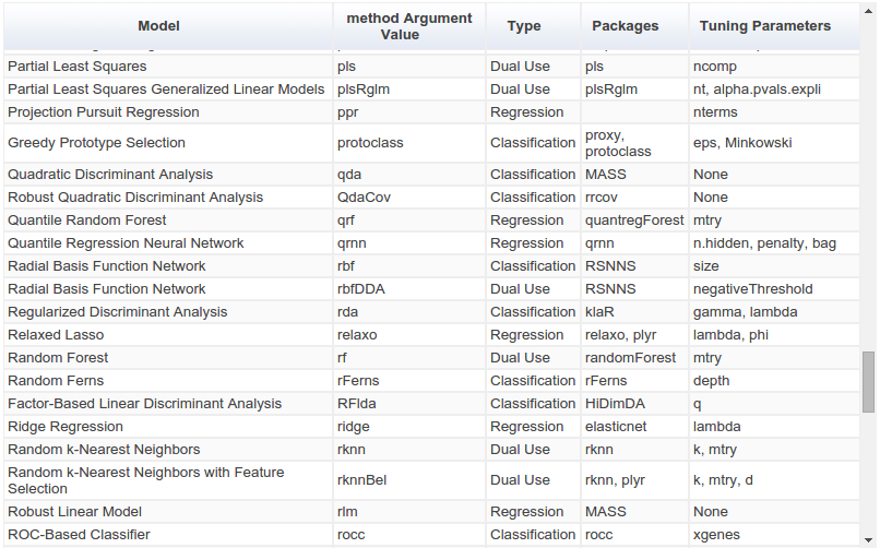
The `caret` package (short for Classification And REgression Training) is a set of functions that attempt to streamline the process for creating predictive models. [...] There are many different modeling functions in R. Some have different syntax for model training and/or prediction. The package started off as a way to provide a uniform interface the functions themselves, as well as a way to standardize common tasks (such parameter tuning and variable importance).
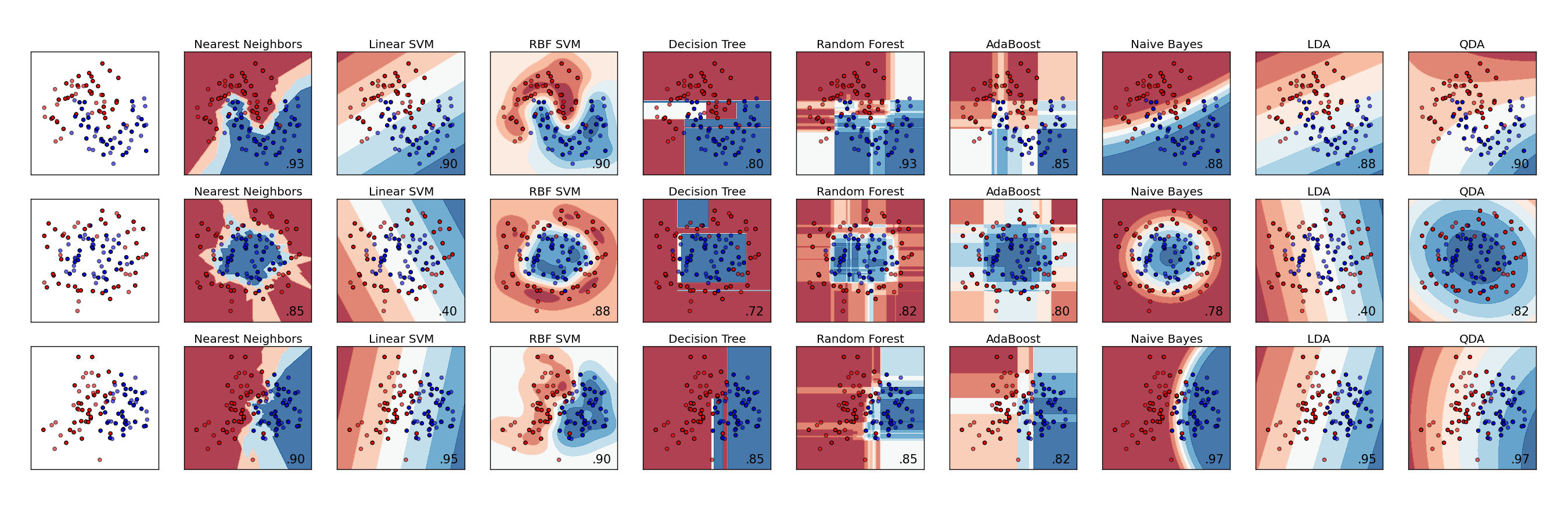
scikit-learn's approach
![]()
Consistent API with a cohesive "grammar" of modeling actions:
Nouns
- Model classes
- Metrics classes
- Preprocessing classes
- Data (as numpy arrays)
- ...
Verbs
fittransformfit_transformscorepredict- ...
![]()
Example problem description:
We'll be using data on blood donations from the UC Irvine Machine Learning Repository. Given some data on some blood donors' previous donations, we'll be trying to predict a binary outcome of whether the donor gave blood in a certain time period.
Here's the official description:
To demonstrate the RFMTC marketing model (a modified version of RFM), this study adopted the donor database of Blood Transfusion Service Center in Hsin-Chu City in Taiwan. The center passes their blood transfusion service bus to one university in Hsin-Chu City to gather blood donated about every three months. To build a FRMTC model, we selected 748 donors at random from the donor database. These 748 donor data, each one included R (Recency - months since last donation), F (Frequency - total number of donation), M (Monetary - total blood donated in c.c.), T (Time - months since first donation), and a binary variable representing whether he/she donated blood in March 2007 (1 stand for donating blood; 0 stands for not donating blood).
Source: https://archive.ics.uci.edu/ml/datasets/Blood+Transfusion+Service+Center
Get the data
From beginning to end, we'll treat the raw data as immutable and base all of our analyses on views and transformations of this "ground truth" data set.
!wget -nc --directory-prefix data \
    https://archive.ics.uci.edu/ml/machine-learning-databases/blood-transfusion/transfusion.data
!head data/transfusion.data
Import the data as a pandas DataFrame
import numpy as np
import pandas as pd

df = pd.read_csv('data/transfusion.data')
df.head()
df.shape
df.dtypes
# save the current names in case we need them later
original_column_names = df.columns

# make the names less ugly
names = ['recency', 'frequency', 'cc', 'time', 'donated']
df.columns = names

df.head()
Some exploratory visualization
# import our graphics tools
%matplotlib inline
import matplotlib as mpl
from matplotlib import pyplot as plt
import seaborn as sns  # nice defaults for matplotlib styles
set2 = sns.color_palette('Set2')

# add on some settings from 'Bayesian Methods for Hackers'
plt.style.use('bmh')

# set larger default fonts for presentation-friendliness
mpl.rc('figure', figsize=(10, 8))
mpl.rc('axes', labelsize=16, titlesize=20)
from pandas.tools.plotting import scatter_matrix

axeslist = scatter_matrix(df, alpha=0.8, figsize=(10, 10))
for ax in axeslist.flatten():
    ax.grid(False)

import numpy as np

# create a figure with 4 subplots
fig, axs = plt.subplots(nrows=2, ncols=2)

feature_column_names = df.columns[:-1]
label_column_name = df.columns[-1]

for i, col in enumerate(feature_column_names):

    # get the current subplot to work on
    ax = axs.ravel()[i]

    # create some random y jitter to add
    jitter = np.random.uniform(low=-0.05, high=0.05, size=len(df))

    # plot the data
    ax.scatter(x=df[col], y=df[label_column_name] + jitter,
               c=df.donated, cmap='coolwarm', alpha=0.5)

    # label the axes
    ax.set_xlabel(col)
    ax.set_ylabel(label_column_name)

plt.tight_layout()
plt.show()

Common tasks with scikit-learn:
Split the data into train and test
from sklearn.cross_validation import train_test_split

# using conventional sklearn variable names
X = df[feature_column_names].astype(float)
y = df.donated.ravel()

# break up the data into train and test
X_train, X_test, y_train, y_test = train_test_split(X, y, test_size=0.5)
X_train.shape
y_train.shape
X_test.shape
y_test.shape
Fit a simple model using the training data
The basic modeling workflow in sklearn involves instantiating a model object with the desired settings, and then fitting it to given data.
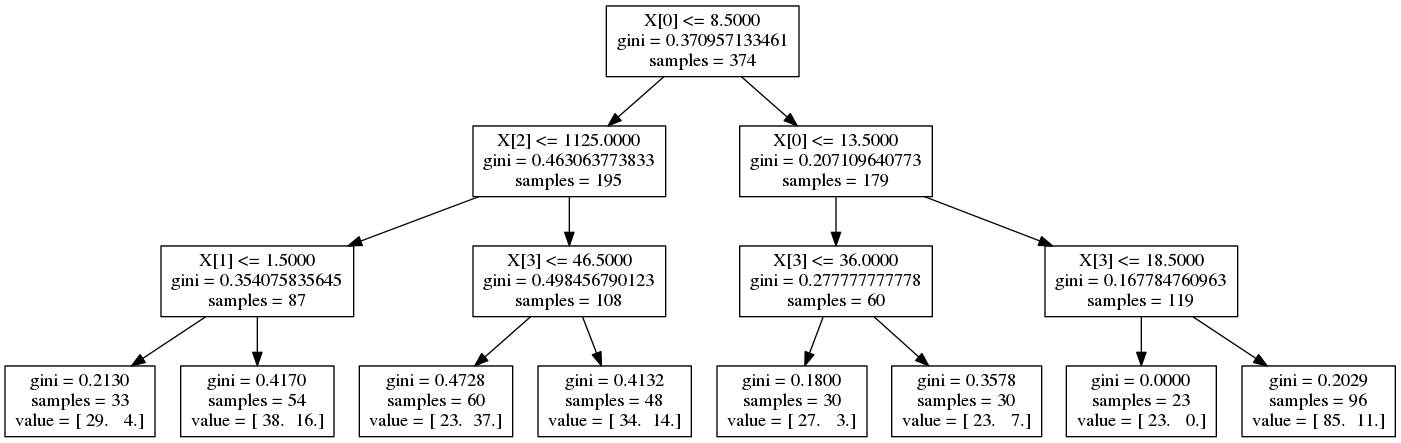
Decision tree
from sklearn.tree import DecisionTreeClassifier

clf_tree = DecisionTreeClassifier(max_depth=3)
clf_tree.fit(X_train, y_train)
print 'Score:', clf_tree.score(X_test, y_test)
# viz adapted from http://scikit-learn.org/stable/modules/tree.html
import pydot
from sklearn.externals.six import StringIO
from sklearn.tree import export_graphviz

dot_data = StringIO()
export_graphviz(clf_tree, out_file=dot_data)
graph = pydot.graph_from_dot_data(dot_data.getvalue())
graph.write_png('output/decision_tree.png')
Logistic regression
from sklearn.linear_model import LogisticRegression

clf = LogisticRegression(penalty='l2', fit_intercept=True)
clf.fit(X_train, y_train)
print 'Score:', clf.score(X_test, y_test)
Trying a bunch of different models
sklearn tries to use the same syntax for most modeling tasks, so it's pretty easy to plug and play.
from sklearn.ensemble import AdaBoostClassifier
from sklearn.ensemble import RandomForestClassifier
from sklearn.naive_bayes import MultinomialNB
from sklearn.neighbors import KNeighborsClassifier
from sklearn.svm import LinearSVC

other_clfs = {
    'Random forest': RandomForestClassifier(),
    'AdaBoost': AdaBoostClassifier(),
    'Naive Bayes': MultinomialNB(),
    'Linear SVC': LinearSVC(),
    'KNN': KNeighborsClassifier(5),
}

# iterating through all of these models we want to fit ...
for name, other_clf in other_clfs.iteritems():

    # fit the model with the training data
    print other_clf.fit(X_train, y_train)

    # cross validation score
    print '---\nScore:', other_clf.score(X_test, y_test)
    print '\n'
Anatomy of a scikit-learn model
The object itself:
clf
Coefficients (if fit):
clf.coef_
Intercept (if fit):
clf.intercept_
Model parameters:
clf.get_params()
Making predictions for $\hat y$:
clf.predict(X_test)
Predicting probabilities, $p(y_i = 1)$
pd.DataFrame(clf.predict_proba(X_test))\
    .head(10)

Challenge: evaluating model performance
The default metric for logistic regression is mean accuracy:
$$\mathrm{accuracy}(y, \hat y) = \frac{1}{n} \sum_{i=1}^n \mathbb{I}(\hat y_i = y_i)$$clf.score(X_test, y_test)
But what if we want a more holistic view of how well this model works?

Common solution: use cross validation tools and other metrics
Cross validation
Our data set here is fairly small $(N=748)$, so what if we happened to randomly pick a non-representative chunk for testing?
Instead of summarizing the performance just on the test data we want to use $k$-fold cross-validation, splitting the data randomly into chunks — "folds" — and evaluating on each to get an idea of the variation in performance.
from sklearn import cross_validation

# come up with random folds of the data
kf = cross_validation.KFold(len(X), n_folds=5, shuffle=True)

def plot_scores(scores):
    N = len(scores)
    plt.bar(np.arange(1, N + 1) - 0.4, scores, color=set2[2])
    plt.title('{}-fold cross-validation scores'.format(N), fontsize=18)
    plt.xlabel('fold', fontsize=14)
    plt.ylabel('score', fontsize=14)
    plt.xlim(0.5, N + 0.5)
    plt.ylim(0, 1)
    plt.show()

# evaluate the fitted model on each fold in turn, returns a score for each fold
scores = cross_validation.cross_val_score(clf, X, y, cv=kf, n_jobs=1)

print 'scores:', scores
print 'average score:', np.mean(scores)
plot_scores(scores)

Other metrics
We can try all sorts of other metrics, though, such as log loss:
$$\textrm{LogLoss}(y, \hat y) = - \frac{1}{n} \sum_{i=1}^n \left[ y_i \log(\hat{y}_i) + (1 - y_i) \log(1 - \hat{y}_i)\right]$$from sklearn.metrics import log_loss
log_loss(y_test, clf.predict_proba(X_test))
Or the F1 score:
$$\textrm{F1} = 2 \frac{\textrm{precision} * \textrm{recall}}{\textrm{precision} + \textrm{recall}}$$from sklearn.metrics import f1_score
f1_score(y_test, clf.predict(X_test))
And if we want more than a single quantity summarizing score, sklearn comes with all sorts of helpful tools like confusion_matrix:
from itertools import permutations
from sklearn.metrics import confusion_matrix

# get the raw confusion matrix
cm = confusion_matrix(y_test, clf.predict(X_test))

# create a dataframe
cmdf = pd.DataFrame(cm)
cmdf.columns = map(lambda x: 'pred {}'.format(x), cmdf.columns)
cmdf.index = map(lambda x: 'actual {}'.format(x), cmdf.index)
cmdf
there are many available ...
metrics.accuracy_score, metrics.auc, metrics.average_precision_score, metrics.classification_report, metrics.confusion_matrix, metrics.f1_score, metrics.fbeta_score, metrics.hamming_loss, metrics.hinge_loss, metrics.jaccard_similarity_score, metrics.log_loss, metrics.matthews_corrcoef, metrics.precision_recall_curve, metrics.precision_recall_fscore_support, metrics.precision_score, metrics.recall_score, metrics.roc_auc_score, metrics.roc_curve, metrics.zero_one_loss, metrics.explained_variance_score, metrics.mean_absolute_error, metrics.mean_squared_error, metrics.r2_score, metrics.adjusted_mutual_info_score, metrics.adjusted_rand_score, metrics.completeness_score, metrics.homogeneity_completeness_v_measure, metrics.homogeneity_score, metrics.mutual_info_score, metrics.normalized_mutual_info_score, metrics.silhouette_score, metrics.silhouette_samples, metrics.v_measure_score, metrics.consensus_score, metrics.pairwise.additive_chi2_kernel, metrics.pairwise.chi2_kernel, metrics.pairwise.distance_metrics, metrics.pairwise.euclidean_distances, metrics.pairwise.kernel_metrics, metrics.pairwise.linear_kernel, metrics.pairwise.manhattan_distances, metrics.pairwise.pairwise_distances, metrics.pairwise.pairwise_kernels, metrics.pairwise.polynomial_kernel, metrics.pairwise.rbf_kernel, metrics.pairwise_distances, metrics.pairwise_distances_argmin, metrics.pairwise_distances_argmin_min... and they all use the same basic syntax.
Refining the model and preparing the data
Challenge: finding reasonable model parameters
The regularization constant, $C$, is unknown. Let's say we want to try some different orders of magnitude as well experimenting with L1 regularization (default for sklearn logistic regression is L2):
We know that the outcome can be different depending on what settings we choose.
Common solution: grid search
From sklearn, we get built in grid search for exploring the space. Using grid search cross validation, we can try all combinations, and automatically keep the most performant.
from sklearn.grid_search import GridSearchCV

params_to_try = {
    'C': [0.01, 0.1, 1, 10, 100, 100],
    'penalty': ['l1', 'l2']
}

gs = GridSearchCV(clf, param_grid=params_to_try, cv=5)
gs.fit(X, y)
print "Best parameters:", gs.best_params_
print "Best score:", gs.best_score_
Challenge: data transformations often needed
One thing we might want to do is scale all of the data before fitting any models. As the sklearn docs point out:
Standardization of datasets is a common requirement for many machine learning estimators implemented in the scikit: they might behave badly if the individual feature do not more or less look like standard normally distributed data: Gaussian with zero mean and unit variance.
Common solution: use plug-and-play data prep tools
It's painful and error prone to wing it every time we want to do common transformations. The sklearn toolbox comes with many useful tools for doing this in a consistent way.
Scaling
from sklearn.preprocessing import StandardScaler

scaler = StandardScaler()

X_train_standardized = scaler.fit_transform(X_train.astype(np.float))
X_train_standardized
print 'column means:', np.round(X_train_standardized.mean(axis=0))
print 'column variances:', np.round(X_train_standardized.var(axis=0))
Now that the scaler is fit on the training data, we can use it to transform new data:
X_new = np.array([25., 35., 9200., 90.])

scaler.transform(X_new)
from sklearn.decomposition import PCA

# instantiate the PCA transformation object
pca = PCA(n_components=2, whiten=True)

# fit the PCA object on and transform the training data
X_train_pca = pca.fit_transform(X_train_standardized)

# create a 3d figure
fig = plt.figure()
ax = fig.add_subplot(111)

# scatterplot the PCA points
ax.scatter(*np.hsplit(X_train_pca, 2), c=y_train, s=40,
           cmap='coolwarm')

# annotate and show the figure
ax.set_xlabel('component 1')
ax.set_ylabel('component 2')

plt.show()

Challenge: all the different steps add up into a big jumbled mess
We have all seen the data science version of this:

But there's no reason for **data_aug_13_v2_scaled_pca_3_dims_WHITENED_plus_some_tweaks_final_V4_FINAL.csv**, right?
We shouldn't have to do that.
Common solution: putting all the steps together with a Pipeline
One big takeaway: it's all about documented, repeatable data-to-model pipelines.
At some point, especially for tasks we will be doing more than once, we might want to codify all of the exploratory work we've done. The standard way to express a beginning-to-end data transformation and model fitting workflow in sklearn is the Pipeline.
from sklearn.pipeline import Pipeline

# define a pipeline with some transforms and a simple classifier
pipeline = Pipeline([
    ('scale', StandardScaler()),
    ('reduce_dim', PCA()),
    ('clf', LogisticRegression()),
])
m
# enumerate all of the different settings we wish to try out
parameters = {
    'reduce_dim__n_components': (1, 2, 3),
    'reduce_dim__whiten': (True, False),
    'clf__penalty': ('l1', 'l2'),
    'clf__C': (1e-3, 1e-2, 1, 1e1, 1e2, 1e3),
}

# grid search the parameter space
grid_search = GridSearchCV(pipeline, parameters, n_jobs=1, verbose=1)

print("Performing grid search...\n")
print("pipeline:", [name for name, _ in pipeline.steps])
print("parameters:")
print(parameters)
grid_search.fit(X, y)

print("Best score: %0.3f" % grid_search.best_score_)
print("Best parameters set:")
best_parameters = grid_search.best_estimator_.get_params()
for param_name in sorted(parameters.keys()):
    print("\t%s: %r" % (param_name, best_parameters[param_name]))
Takeaways for using sklearn in the real world
- API consistency is the "killer feature" of
sklearn - Treat the original data as immutable, everything later is a view into or a transformation of the original and all the steps are obvious
- To that end, building transparent and repeatable dataflows using Pipelines cuts down on black magic
Public service announcement: using other tools
Why choose? Use whichever one is best for the task at hand.
# load the %R cell magic extension
%load_ext rmagic

# send the dataframe over to the R instance
%Rpush df
%%R
library(ggplot2)
qplot(log(time), log(cc), data=df, color=donated)

%%R
blood.glm <- glm(donated ~ log(cc) + log(time), data=df, family="binomial")
print(summary(blood.glm))

par(mfrow=c(2, 2))
plot(blood.glm)

... and we can pull data back from R to Python:
r_coeffs = %R coef(blood.glm)
r_coeffs
Even better for those in the Julia community ... you can replicate this whole experience when working in an IJulia notebook:

In fact - IPython notebooks are not just for Python anymore. The core functionality has been generalized as Project Jupyter, and language kernels are available or under active development for Julia, Haskell, and R.