I finally got rid of my car earlier this year. It served me well, but I currently live in the city and take the subway most of the time. Now that it's gone, it's time to take a look at the data.
From when I bought the car used in 2009 until I sold it this past summer, I made a log entry every time I refueled the car. (I realize this is not normal.)
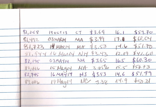
I noted the date, mileage on the odometer, number of gallons of gas I bought, and the price of gas. Every now and then I'd remember to bring in the log and update my spreadsheet on Google Docs. Here's what the data looks like after being downloaded as a csv.
!head data/jeep.csv
Let's read it in and get going.
%matplotlib inline
from matplotlib import pyplot as plt
import seaborn as sns
plt.style.use('fivethirtyeight')

import numpy as np
import pandas as pd

df = pd.read_csv('data/jeep.csv', parse_dates=['date'])
df.head()
df.info()
Looks like the miles column was read in as strings (its dtype is object), so we just need to fix that:
# remove commas and cast to int type
df.miles = df.miles.str.replace(',', '').astype(int)
df.info()
Miles driven
Let's look at the mileage over time. I bought the car used, so the mileage starts near 40,000.
# use friendly commas for thousands
from matplotlib.ticker import FuncFormatter
commas = FuncFormatter(lambda x, p: format(int(x), ','))

plt.plot(df.date, df.miles)
plt.xlabel('date')
plt.ylabel('mileage')
plt.gca().get_yaxis().set_major_formatter(commas)
plt.show()

Mileage per gallon
One quantity of interest to car buyers is fuel efficiency. Without knowing much about cars, I'd assume that as components age the mileage per gallon (MPG) will decline. Let's see if that's the case. The first thought on how to do this would be
$$\frac{\textrm{miles driven since last fill-up}}{\textrm{gallons purchased last time}}$$but the fill-ups came at irregular intervals and weren't always up to a full tank, so these fractions could be all over the place. Instead, we can divide the cumulative sum of miles driven by the cumulative amount of gasoline purchased. The first few numbers will be crazy but it will pretty quickly converge to a reasonable estimate.
# add a miles per gallon series
df['mpg'] = df.miles.diff().cumsum() / df.gal.cumsum()

# plot the points
plt.scatter(df.miles, df.mpg, c='#30a2da')

# plot the exponentially weighted moving average of the points
plt.plot(df.miles, pd.ewma(df.mpg, 5), lw=2, alpha=0.5, c='#fc4f30')

# ignore the first handful of these
plt.xlim(45000, df.miles.max())
plt.ylim(17, 21)

plt.xlabel('mileage')
plt.ylabel('mpg')
plt.show()

A couple of interesting notes here:
- The dots that are unusually high probably correspond with long highway drives.
- As for the discontinuity around 54,000 miles, I figured out by looking through my car folder that this was when I replaced the tires. It's possible that the new tires had higher drag causing lower fuel efficiency.
Fitting a simple model
It could be interesting to quantify how fuel efficiency changed as the car aged.
import statsmodels.formula.api as smf

# create a new view into the old dataframe for fitting
# (throw away the first 30 points)
model_df = df.ix[30:, ['miles', 'mpg']].copy()

# divide the new miles by 10k so the regression coefficients aren't tiny
model_df.miles /= 1e4

# fit the model
results = smf.ols('mpg ~ miles', data=model_df).fit()

# print out results
results.summary()
It looks like my fuel efficiency went down about 0.44 miles/gal for every 10,000 miles of wear and tear.
Miles driven per year compared to US average
First, we'll sum up the data grouped by year.
driven_per_year = df.set_index('date').miles.diff().resample('1A', how='sum')
driven_per_year
Next, we'll grab annual driving stats from the Federal Highway Administration, an agency of the U.S. Department of Transportation.
# use `read_html` to get the <table> element as a DataFrame
parsed_tables = pd.read_html('https://www.fhwa.dot.gov/ohim/onh00/bar8.htm', header=0)
us_avg_miles = parsed_tables.pop().set_index('Age')
us_avg_miles
driven_per_year / us_avg_miles.ix['20-34', 'Male']
So it looks like I drive less than average. This makes sense — from 2008 until mid-2010, I spent about half the year at sea with my car sitting on the pier. In 2010, I moved back to Boston and my primary mode of transportation was walking or taking the T.
Gas prices
Even without driving that much, it's possible to spend quite a bit on gas.
plt.plot(df.date, (df.gal * df.price).cumsum(), label='cumulative dollars spent on gas')
plt.plot(df.date, df.gal.cumsum(), label='cumulative gallons gasoline bought')

plt.xlabel('date')
plt.gca().get_yaxis().set_major_formatter(commas)

plt.legend()
plt.show()

Thanks to the Energy Information Administration, an entity within the U.S. Department of Energy, it's also possible to compare the prices at which I bought gas to the national average price over time.
!wget -O data/gas.xls http://www.eia.gov/dnav/pet/xls/PET_PRI_GND_DCUS_NUS_W.xls
It's an Excel file, unfortunately, but pandas makes it easy to get at the data. I opened Libreoffice just to see how it's laid out, then read it in with the read_excel method.
gas = pd.read_excel('data/gas.xls', sheetname='Data 1', header=2)
gas.info()
From here, we'll narrow the national gas data down to just the part we care about (regular gasoline) and plot it alongside what I paid.
# slice off the data we care about
regular = gas[['Date', 'Weekly U.S. Regular All Formulations Retail Gasoline Prices  (Dollars per Gallon)']]
regular.columns = ['date', 'usa_avg_price']

# plot the two trends
plt.plot(df.date, df.price, label='dollars per gallon paid')
plt.plot(regular.date, regular.usa_avg_price, lw=2, label='national avg')

# annotate the figure
plt.xlabel('date')
plt.ylabel('gas price per gallon (USD)')
plt.xlim(df.date.min(), df.date.max())

plt.legend()
plt.show()

I was usually filling up in New England which is probably a little more expensive than the national average.
In closing
Not exactly the most hard hitting blog entry of all time, but I spent a bunch of time over the years writing it all down so... may as well make some plots!
Aside: for anyone considering keeping a log in your car, keep in mind that you will take a lot of flak from passengers. Think about it.