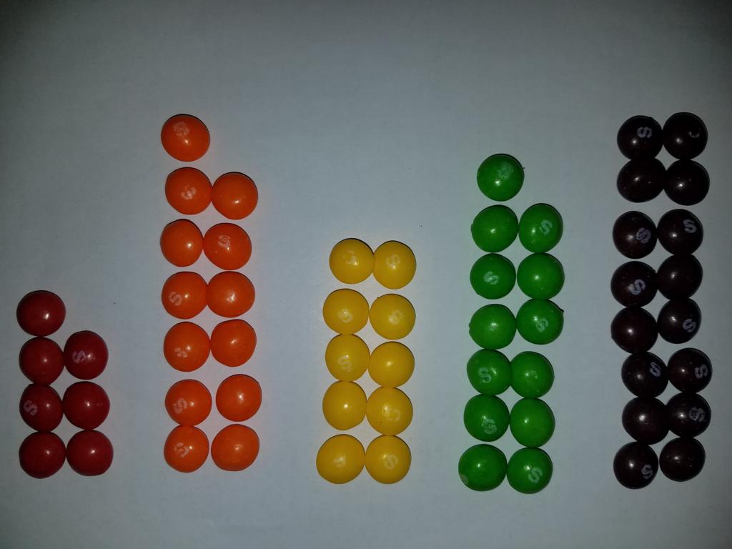
Last year I came across a blog post describing how the author collected count data from 468 packs of Skittles. (It's a great blog post, definitely worth reading.) For each bag, the author counted up how many of each color were present.
Using data from the Github repo for the project, we can fit a Bayesian model to see what the underlying proportions of each color might be.
Reading in the data
%matplotlib inline
from matplotlib import pyplot as plt
import seaborn as sns
import numpy as np
import pandas as pd

import warnings
warnings.filterwarnings("ignore")

skittles_palette = ["red", "orange", "yellow", "green", "purple"]

df = pd.read_csv("../data/skittles.txt", sep="\t").drop("Uncounted", axis=1, errors="ignore")
df.head(10)
df.shape
We can also normalize each row by its sum (the total number of skittles in that bag) to show the proportion of each color in the bag:
counts = df.sum(axis="columns")
normalized = df.div(counts, axis="rows")
normalized.head()
Exploratory analysis
Now that we have the data, we can ask a few simple questions just with descriptive statistics and visualizations. Here's an attempt at a quick summary of the whole data set all in one picture:
def summary_plot():
    fig, ax = plt.subplots(figsize=(10, 20))

    # plot the mean for each color
    for i, cumulative_mean in enumerate(df.mean(axis="rows").cumsum().values):
        color = df.columns[i]
        label = f"mean={df[color].mean():0.2f}"
        plt.axvline(cumulative_mean, c=skittles_palette[i], alpha=0.5, lw=2, label=label)

    # draw stacked bars
    _sorted_index = df.sum(axis=1).argsort()[::-1]
    df.loc[_sorted_index].plot(kind="barh", stacked=True, ax=ax, color=skittles_palette)


    # plot the overall mean
    _overall_mean = df.sum(axis="columns").mean()
    _jitter = 0.2
    plt.axvline(
        _overall_mean + _jitter,
        c=skittles_palette[-1],
        alpha=0.5,
        ls="--",
        label=f"mean total={_overall_mean:0.2f}"
    )

    ax.set_yticks([])
    ax.xaxis.tick_top()
    plt.tick_params(axis="x", top=True)
    sns.despine()
    plt.legend(loc="upper right")
    plt.show()

summary_plot()

How many skittles are usually in a bag?
sns.distplot(counts, bins=31)
sns.despine()
plt.xlim(50, 70)
plt.show()

How many of each color are usually in a bag?
def plot_counts(axs):
    ax = axs[0]
    sns.boxplot(
        data=pd.melt(df, var_name="color", value_name="count"),
        x="color",
        y="count",
        palette=skittles_palette,
        ax=ax
    )
    sns.despine()
    ax.set_title("counts per bag")

    ax = axs[1]
    for i, color in enumerate(df.columns):
        sns.distplot(df[color], color=skittles_palette[i], ax=ax, hist_kws={"alpha": 0.1})
    sns.despine()
    ax.set_xlabel("count")


fig, axs = plt.subplots(ncols=2, figsize=(14, 4))
plot_counts(axs)
plt.show()

What about the observed proportions?
def plot_proportions(axs):
    ax = axs[0]
    # counts
    sns.boxplot(
        data=normalized.melt(var_name="color", value_name="proportion"),
        x="color",
        y="proportion",
        palette=skittles_palette,
        ax=axs[0]
    )
    ax.set_ylim(0, 0.4)
    sns.despine(ax=ax)
    ax.set_title("proportions per bag")

    ax = axs[1]
    for i, color in enumerate(normalized.columns):
        sns.distplot(normalized[color], color=skittles_palette[i], ax=ax, hist_kws={"alpha": 0.1})
    sns.despine()
    ax.set_xlim(0, 0.4)
    ax.set_xlabel("proportion")

fig, axs = plt.subplots(ncols=2, figsize=(14, 4))
plot_proportions(axs)
plt.show()

These graphs give a descriptive feel for the data, but we can't yet draw more general conclusions. That's a job for statistical inference.
Inference: what are the true proportions for each color?
We can assume that the manufacturer is motivated to control the average number of Skittles per bag for cost and packing reasons. What is less clear is whether they exert any intentionality over the proportion of colors.
One thing we might want to look into: are the proportions for each color in a bag supposed to be the same or are any flavors purposely favored or disfavored? And if the differences are intentional, what are the intended proportions for each color?
Eyeballing the plot above, we might hypothesize that the machines are trying to get about 20% of each color and that fluctuations are due to machinery imprecision. For example, it is possible that it is solely due to random fluctuations that we see slightly more lemon and slightly less apple. The means give us our maximum likelihood estimate (MLE) for the "true" proportions:
normalized.mean(axis="rows")
The MLE converges on the true population values given infinite trials, but how do we know how different the real population was given we have observed only $N=468$ trials?
The frequentist attempt to answer the question might use a null hypothesis significance test (NHST) where the null hypothesis is that the proportions are the same. For this scenario the standard test would be a one-way ANOVA, which is sort of like a Student's t-test generalized to more than two groups:
import statsmodels.api as sm
from statsmodels.formula.api import ols

melted_proportions = normalized.melt(var_name="color", value_name="proportion")
model = ols("proportion ~ color", data=melted_proportions).fit()
sm.stats.anova_lm(model, typ="II")
This p-value of $0.0005$ is very small, telling us that if the null hypothesis were true then we would be very unlikely to see data with differences in means (as captured by the F statistic) as extreme or more extreme than what we actually saw in our sample. Since $p < 0.05$ or some other small-ish number we would reject the null hypothesis and conclude that the intended proportions of each color are probably not the same.
A couple notes about this test:
- It doesn't really tell us what we want to know. The test only tells us that not all of the proportions are exactly the same. It doesn't tell us which ones are different and by how much. If you wanted to know about individual differences you would have to do a bunch of pairwise comparisons which is a recipe for falsely finding significance by random chance.
- It doesn't quantify our remaining uncertainty about the estimates. When we take the mean of each color, that MLE is a point estimate: one single number that represents the whole group. We know that this estimate is subject to randomness, so how much plausibility do we allocate to higher or lower values?
Both of these drawbacks are typical motivations for fitting a Bayesian model that more fully characterizes the data generating process.
Choosing the Dirichlet-multinomial
In order to build a Bayesian model, we need to come up with a believable data generating process, which is a story of how our data came to be. Here's one for the Skittles data:
- The factory decides on a proportion of Skittles $\mathbf{p} \in \mathbb R^5$ where each $p_j \geq 0$ and they sum up to 1.
- The factory makes a large number of Skittles in these proportions and then mixes them all up into a big hopper.
- For each bag $i$, the Skittles factory selects a number of Skittles $n$ to put in that bag.
- Then the factory draws $n$ Skittles from the big hopper and puts them into the bag, and it turns out that a count $k_j$ of each color is observed in the bag.
This corresponds almost exactly to the Dirichlet-multinomial model, where the Dirichlet is the prior distribution over proportions and the multinomial is the distribution for counts of each group. (This is the generalization of the Beta-Binomial model which does the same but for only two groups, e.g. heads versus tails on flips of a biased coin.) In particular, having proportional amounts of Skittles in a hopper ready to dispense corresponds directly to the Pólya urn interpretation with an extemely large $K$.
The Dirichlet gives us a distribution over simplexes (vectors that add up to one), and the multinomial gives us a distribution over an enumerated set of discrete outcomes. Together, we have a model for the proportions which we can condition on the observed data. Based on the question we're asking above, the parameter we are most interested in is the $p$ parameter of the multinomial which is sampled from the Dirichlet prior - or the idealized proportions for each color before they are probabilistically sampled into actual counts.
Here's how we could set this up in PyMC3:
import pymc3 as pm
import arviz as az

color_names = df.columns

with pm.Model() as model:
    # make the Dirichlet an uninformative prior
    alpha = np.ones(len(color_names))
    # choose true proportions
    p = pm.Dirichlet("p", a=alpha)
    # choose a bag size
    n = pm.DiscreteUniform("n", lower=40, upper=100, observed=df.sum(axis=1).values)
    # choose how many of each color to put in that bag adding up to n based on proportions p
    k = pm.Multinomial("k", n=n, p=p, observed=df)

    trace = pm.sample(2500)
    fit = az.from_pymc3(trace=trace, coords={"p_dim_0": color_names})
Setting the $\alpha$ parameter of the Dirichlet to ones makes it a uniform prior over simplexes, so it's uninformative here. In any case there's probably plenty of data to overwhelm whatever reasonable prior we would set.
Diagnostics
There were no divergences during sampling, so that is good. But before we draw any conclusions from the model, we should check to make sure the sampling went well. Having sampled 4 chains of 2,500 iterations each, we can use arviz to look at the summary:
summary_df = az.summary(fit).reset_index().assign(color_name=df.columns).set_index("color_name")
summary_df
Here, we can see the summary stats for our estimates of each parameter. Especially of note:
- The Gelman-Rubin $\hat R$ statistic (
r_hat) is less than 1.01 for each parameter indicating that we don't have signifcant divergence between chains. - The tail effective sample size (
ess_tail) is still in the high thousands meaning we have probably explored the parameter space pretty well.
We can also look at the traceplot for the MCMC sampling:
az.plot_trace(fit)
plt.show()

On the left, we see that each of the 4 chains generally agreed with all the others for each of the parameters. On the right, we see nice "fuzzy caterpillars" indicating that chains didn't get stuck in any proposals.
Getting our answers from the trace
Let's look at what our MCMC chains say about these parameters. We'll look at the 89% credible interval after McElreath, who suggests 89% in "Statistical Rethinking" because (1) unlike 95% or other neat numbers we are used to seeing, 89% is a little weird so it reminds us that it's an arbitrary choice, and (2) it's prime making it slightly special, so why not.
az.plot_forest(fit, credible_interval=0.89)
plt.show()

This plot nicely shows the uncertainty around each maximum a posteriori (MAP) estimate with four lines per parameter, one per MCMC chain. They are all aligned on the same x axis this time, so we can clearly see which ones overlap and which ones do not.
As we can see, our credible interval for apple does not overlap with lemon or grape at all, which means we don't believe that we could have observed the data we collected if the underlying proportions were actually the same.
A different data story
In the Dirichlet-multinomial model, we imagined a giant hopper where all the colors were mixed up and then sampled into a noisy bag size. We tried to learn $p$ while throwing away the distribution over bag sizes as a nuisance parameter.
The thing is, we might not be right about this — what if all the colors are kept separate, and the way the bag is filled is just 5 independent attempts to put roughly $μ_i$ in the bag from each color $i$ plus or minus machine error $\sigma$?
The nice thing about Bayesian models is that we can try to model this story directly:
with pm.Model() as model2:
    # error, centered at zero with a large sigma to make this prior pretty uniformative
    sd = pm.HalfNormal("σ", sigma=5.0)
    # mu vector with 5 entries that we are trying to fit; use a Normal as the natural
    # representation of an expected value with random errors
    mu = pm.Normal(f"μ", mu=10, sigma=2, shape=df.shape[1])
    for i, color in enumerate(df.columns):
        # condition each color's mu with the observed counts for that color
        n_i = pm.Normal(f"n_{color}", mu[i], sd, observed=df[color])

    trace2 = pm.sample(2_500)
    fit2 = az.from_pymc3(trace=trace2, coords={"μ_dim_0": color_names})
az.summary(fit2)
az.plot_trace(fit2)
plt.show()

az.plot_forest(fit2, var_names=["μ"], credible_interval=0.89)
plt.show()

Nicely, this result is pretty similar to the above model even though it's describing a much different story. It confirms that apple has a substantially different underlying probability.
Conclusion
Most notably, we can conclude that apple really is less present than all the other colors by an average of one Skittle per bag.
In actual inference, we might want to compare these models using LOO or WAIC. But that's probably enough for Skittle modeling.