Here's another nice PuzzlOR problem which lets us look at different ways to tackle an optimization problem, including deterministic and stochastic approaches.

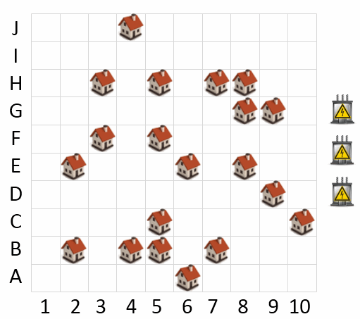
A new city is being built which will include 20 distinct neighborhoods as shown by the house icons in the map. As part of the planning process, electricity needs to be connected to each of the neighborhoods.

The city has been allocated funds to put in 3 electrical substations to service the electrical needs of the neighborhoods. The substations are represented by the 3 electrical box icons to the right of the map. Because laying electrical line to each neighborhood is expensive, the placement of the substations on the map requires careful consideration.

A neighborhood will be serviced by the nearest electrical substation. A neighborhood may only be connected to one substation. The substations may be placed in any cell (including the same cell as an existing neighborhood). The cost of electrical wiring is $1M per km. Distances are measured using a direct line between cells, which are each 1km apart. For example, the distance between cell A1 and B2 is 1.41km.

Question: What is the minimum cost required to connect all neighborhoods to electricity?

Problem set-up¶

We'll import the necessary libraries and write some utility functions for modeling this problem.

Here are the starting positions of the neighborhoods in array form:

As in any optimization problem, we wish to minimize some loss function. Here we are trying to minimize a cost defined as a constant times a sum of distances, so the main building block for our loss function will actually be a distance metric. We will define a function that, given an $(x,y)$ power plant coordinate $s$ and a collection of $(x,y)$ neighborhood coordinates $N$, will return an array of Euclidean distances between the power plant $s$ and each neighborhood $n \in N$.

As an example usage, plugging in $(5,5)$ for a single power plant will return the distances from that point to every single neighborhood:

As usual, we'll represent our problem in matrix form as a convenient way to assemble many simultaneous pieces of information at once. To that end, we'll build on our previous function and define a new one that takes a collection of power plant $(x,y)$ coordinates and returns a matrix of every power plant-neighborhood distance.

Each row will correspond to one power plant location, and each column will correspond to one neighborhood location. Practically speaking, we are simply stacking rows from the function above.

And here is an example usage, picking some arbitrary starting points.

In this problem, the distance (or loss) for each neighborhood is based on the closest power plant; anything farther away doesn't matter. We can think of this as the closest power plant to a neighborhood being responsible for that neighborhood.

Here we'll define a function which takes the $S \times N$ matrix of distances from each power plant $s$ to each neighborhood $n \in N$, and return an array that tells us which power plant is responsible for each neighborhood.

Having done that footwork, we can get to the heart of the issue: what is the sum of distances from each power plant to the neighborhoods for which it is responsible?

The total loss is just the sum of those sums times a constant of \$1,000,000 which we will ignore. For certain applications, loss is thought of as the *energy state* of the system (lower is better). Simulated annealing is one of those, so we'll go by that convention and call the loss function $E$.

We now have everything necessary to solve this problem: constraints, decision variables, and a loss function (or "objective function").

That being said, it's helpful to picture what's going on in the problem for at least two reasons—as a sanity check to make sure that there aren't any obvious bugs, and to solidify intuition about what's actually happening. Here's a function that will take some power plant placements, the fixed data about where neighborhoods are, and depict distances between power plants and the neighborhoods for which they are responsible.

How to solve it¶

First of all, this problem is a clear cut instance of a combinatorial optimization problem. We have 100 places to put power plants, and can think of having 100 decision variables $x_{ij} \in \{0,1\}$ for whether or not we have a power plant on that grid point.

While the puzzle we are working on is a toy problem, it is also related to the Euclidean minimum spanning tree and Steiner tree problems, both of which are interesting, important, and used to model real world problems—including power plant placement!

Generally speaking, there are two approaches to this kind of optimization problem: deterministic and stochastic. Deterministic methods include brute force search as well as integer program algorithms such as branch and bound. Popular stochastic optimization approaches include simulated annealing, genetic algorithms, and many other variations on the same idea.

We'll solve it both ways, deterministically and stochastically.

Deterministic approach: brute force¶

The classic approach to solving this kind of integer program (IP) would be to set up the model (constraints, decision variables, and objective function) and use a solver specifically designed for solving linear programs.

Now, we could set up a linear program here. (In a previous post, I showed how to set up and solve a linear program in Python.) But before we do that, let's review a couple of facts about this problem:

• For the grid specified in the problem description, there are $10^2=100$ possible locations to put power plants. Each location's decision variable has two possible states $\{0,1\}$: not having a power plant or having one.

• Without applying any knowledge of constraints (number of power plants, non-colocation), that means there are $2^{100}$ possible configurations. That's more possibilities than there are stars in the universe.

• However, applying the constraints of placing only three power plants and requiring that they be non-colocated, that number decreases to $\dbinom{100}{3}$.

How big is that?

So there are really not that many candidate solutions; our loss function is fast enough that we can just try them all and pick the best.

So now we have an array of all values of the loss function:

Out of curiosity, we can also see how values of this loss function are distributed:

And the reveal: which answer was best?

Or, in our alphanumeric grid system:

And here is what that optimal solution looks like:

So there's the answer. But let's be clear: brute force was only possible here because we're dealing with a tiny feasible region. The computational complexity of brute force search makes it inappropriate for any non-trivial combinatorial optimization problems.

Even if the domain isn't intractably large, a common problem is that the loss function is expensive to run. Ours takes microseconds; what if it took minutes? We would no longer be able to explore exhaustively, instead we would have to sample.

Stochastic approach: simulated annealing¶

Simulated annealing is a powerful stochastic optimization method with deep connections to MCMC. It uses a clever analogy to the physical process of annealing metal as inspiration for choosing acceptance probabilities in the proposal step. There's a ton of great material out there discussing SA, but here are the basic ideas:

• We start at some candidate solution and also initialize a variable to keep track of the best solution we ever saw.

• At each iteration, we propose a new candidate solution by perturbing the current candidate in some way.

• If the proposed solution is better, we always "move" (that is, start using it as the current proposal). If not, we might move anyway because we want to explore the domain; if we're strictly hill-climbing then we risk getting stuck in a local optimum. (This is the fundamental idea of the Metropolis-Hastings algorithm.)

• Our chance of moving to a worse proposal is positively related to the current temperature and negatively related to how much worse the proposal is than the current solution.

• We'll start with a high temperature in order to explore widely, but gradually let the temperature decay so we can focus on optimizing locally.

• Sometimes, we will re-anneal by temporarily bumping the temperature way back up. This is where the metallurgy analogy comes in; in order to bring out flexibility in metals they may be repeatedly heated and cooled.

In this way, SA tries to balance twin goals of (1) exploring widely and (2) squeezing the last bit of optimization out of probable winners.

I'll adapt some simulated annealing Python code from a previous project, available directly as optimization.py in our project's Github repo. Given a loss function (energy), a function to make proposals by perturbing the current state (perturb), and a starting state (n0), this simulated annealing function will continue to explore the problem domain.

So how to perturb the current solution? There are many different ways we could do this. Typically, the best ways will allow enough random change to help explore the domain but preserve some similarity between the current and proposed candidates—otherwise, we're just doing a completely random exploration which defeats the purpose.

Here, we'll perturb the current solution by randomly choosing one of the power plants and adding $\mathcal{N}(0,1)$ noise to its current position.

And now we're ready to go:

Now we can obey the constraints of the original problem by "snapping" the power plants' optimized positions in $\mathbb{R}$ to the closest grid points:

So we got to the brute force solution. How quickly though?

As we can see, this algorithm started getting pretty good answers almost immediately, and fairly quickly converged down towards the optimum. Not only that, we actually found an optimal solution. And it's important to remember that we weren't even perturbing the current candidate in a smart way.

One of the reasons simulated annealing is so widely used is that in practice it's robust over many possible choices of parameters, which include how to make proposals, starting temperature, number of times to re-anneal, fraction of temperature to re-anneal up to, etc.

Curveball solution: using k-means clustering¶

One of the interesting things about this problem is its many connections to other problems. Thinking about what we're really doing as we move the power stations around, it becomes clear that we are trying to break up neighborhoods into 3 clusters and place the power plants as close to the centroid of each cluster as possible.

This is an instance of k-means clustering. Here, $k=3$, and we'll momentarily relax the assumption from the original problem that power plants must be at grid points (we'll fix it later).

Once again, we'll snap these real-valued placements to the nearest grid points to get an acceptable solution:

And again, we arrive at the optimum.